Overview

• topic models were originally designed for information retrieval taks such as finding relevant documents in large online archives as an alternative to keyword-based searches
  • problems of synonymy and polysemy
  • find documents which share the same themes (e.g. politics, business, sports)
• standard methods usually make bag-of-words assumption: word order does not matter (however: n-grams, methods based on Markov chains)
• mainly two branches:
  • linear algebra methods based on dimensionality reduction: LSI (latent semantic indexing)
  • probabilistic methods: pLSA (probabilistic latent semantic analysis) and LDA (latent dirichlet allocation)

Latent Dirichlet Allocation

[1] D. Blei, A. Ng, and M. Jordan, “Latent dirichlet allocation,” J. Mach. Learn. Res., vol. 3, pp. 993–1022, 2003.

• probabilistic graphical model for text documents
• extends the mixture of uni-grams model ("Bayesian naive Bayes") by permitting multiple topics per documents (the former is an example of a clustering method, whereas topic models are subsumed under mixed-membership models)
• wildly popular, mainly because of its expandability

What is Bayesian statistics?

• Eat spaghetti
• Drink wine

Bayes' Rule

\[\definecolor{lviolet}{RGB}{114,0,172} \definecolor{lgreen}{RGB}{45,177,93} \definecolor{lred}{RGB}{251,0,29} \definecolor{lblue}{RGB}{18,110,213} \definecolor{circle}{RGB}{217,86,16} \definecolor{average}{RGB}{203,23,206}\]

\[ {\color{lgreen} P ( \theta | D )} \color{black} = \frac{\color{lblue}P ( D | \theta ) \color{black} \color{lviolet}P( \theta)} {\color{black}P ( D )}\]

Given observations \( D \), we update our beliefs about the parameters \( \theta \) which govern the underlying data generating process. We compute the posterior distribution of the parameters as the product of the likelihood times the prior beliefs about the parameters, suitably normalized.

A simple example

Scenario: We throw a bunch of coins and would like to estimate the probability \( \theta \) of the coin landing on its head. This is a simple sequence of Bernoulli experiments, where \( X_1, \ldots, X_n \sim \operatorname{Bern}( \theta) \). If we throw the coin three times and observe \( D = \{ H,H,H \} \), the likelihood of the data is given by

\[ \color{lblue} P(D|\theta) = \theta^3 (1 - \theta)^0 = \theta^3. \]

The MLE is \( \hat \theta = 1 \). As we can see, the frequentist approach yields point estimates which are entirely driven by the data. In contract, in a Bayesian analysis a prior for \(\hat \theta\) has to be specified.

Bayesian machinery

A beta prior yields tractable results. \[ P(\theta) = \theta^{\alpha - 1} (1 - \theta)^{\beta - 1 } \] The posterior distribution evaluates to \[ P(\theta | D) \propto \theta^{3 + \alpha -1} (1 - \theta)^{ 0 + \beta - 1} \]

The MAP (maximum a posteriori) estimate is then given by \(\hat \theta = \frac{3 + \alpha} {3 + \alpha + \beta}\). With \(\alpha = \beta = 100\), we have \(\hat \theta = \frac{103}{203} \approx 0.5\). Almost no influence of the data! Conclusion: Whereas frequentist point estimates trust entirely the data, Bayesian estimates are conservative in nature: Much more data is required such that the prior beliefs encoded in the prior distribution are washed out. You might ask: What has this to do with the modeling of text documents?

Documents as distributions over words

Generalization of Bernoulli distribution: Multinomial. Assume we have access to a vocabulary of all possible words:

\[ V = \{ \color{circle} Cat \color{black}, Dog, Lunch, \color{average} Mouse \color{black}, \color{lred} Eats \color{black}, \ldots \} \]

We make the bag-of-words assumption: Order of words in a document does not matter. The probability of the text \(D_i = \text{"Cat eats mouse"}\) given the word distribution \(\ {\theta}\) then is \[ P(D_i) \propto \color{circle} \theta_1 \color{black} \cdot \color{lred} \theta_4 \color{black} \cdot \color{average} \theta_5 \]

General Setup

\(K\) Topics, each endowed with word distribution \(\vec \theta_k\). For example, consider again

\[ V = \{ \color{circle} Cat, Dog, \color{lblue} Lunch, \color{circle} Mouse \color{black}, \color{lblue} Eats \color{black}, \ldots \} \]

Then we might have \[ \color{circle} \vec \theta_{\text{Animals}} = (0.2 , 0.2, 0.03, 0.1, 0.05, \ldots) \] and \[ \color{lblue} \vec \theta_{\text{Food}} = (0.03,0.04,0.3,0.07,0.2, \ldots) \]

• Must ensure that each topic assigns positive probability to each word, however small, as otherwise any document will never be assigned to a topic in which one of its words has probability zero.
• Hence, use of Bayesian probability instead of frequentist approach: Recall that the beta distribution is a conjugate prior to the Bernoulli. For more than two classes, the Dirichlet distribution is a conjugate prior for the Multinomial distribution.

Generative Model of LDA

Each document is created as follows:

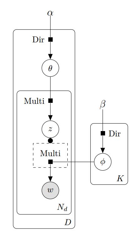
• Draw a distribution over topics \(\theta\) for the document
• For the i-th word in the document, first draw a topic \(z_i\) from \(\theta\)
• Draw the word \(w_i\) from \(\phi_{z_i}\)